| P*1 - P*1(T) = 0 | P y1 - x1 P*1 = 0 | P*2 - P*2(T) = 0 | P y2 - x2 P*2 = 0 | x1 + x2 - 1 = 0 | y1+ y2 - 1 = 0 |
| P*1 - P*1(T) = 0 | (1) | p1 - x1 P*1 = 0 | (2) | P*2 - P*2(T) = 0 | (3) | p2 - x2 P*2 = 0 | (4) | x1 + x2 - 1 = 0 | (5) | p1+ p2 - P = 0 | (6) |
The remaining unknowns in the equations are then:
P , P*1 , p1 , P*2 , x2 , p2
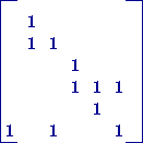
We can draw up an incidence or occurrence table for the set of equations as shown below, with a row for each equation and a column for each unknown, where an `x' indicates that the specified variable occurs in the equation and a blank that it does not.
| Variable: | P | P*1 | p1 | P*2 | x2 | p2 |
| Equation (1) | x | |||||
| Equation (2) | x | x | Equation (3) | x | Equation (4) | x | x | x | Equation (5) | x | Equation (6) | x | x | x |
We might want to write this in `mathematical' notation we would replace the x's by ones, leaving the blanks, which are conventionally taken to imply zeros. The matrix would then look like this:
We explain the use of this type of matrix or table for ordering equations in section 1.1.2.3. To summarise briefly, the matrix shows that equations (1), (3) and (5) contain only a single unknown each, and so can be solved for each of these, i.e. respectively for P*1 , P*2 and x2. It can then be seen that equation (2) now contains only one remaining unknown, p1 as P*1 is no longer unknown, and so it can be solved. In fact all the remaining unknowns can now be determined by solving equation (4) and then (6) each for a single unknown.
Use of the matrix has shown how a problem which might have been thought to involve the simultaneous solution of 6 equations in six unknowns actually involves solving only one equation at a time.