Controller Design and System Modelling

Tuning a Controller

Introduction

In the first section on controllers we looked at two control algorithms for proportional and proportional integral controllers. In order to implement these algorithms there are two parameters which have to be fixed, namely

, the controller gain
, the integral reset time

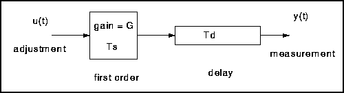
In the second section on modelling processes we looked at

First order input output processes
Mechanistic models of actual processes

For the first of these we saw that there were three parameters necessary to define the process. These are

T, the dead time
, the process gain
, the process time constant

The aim of this section is to introduce a method of matching the personality of the controller to that of the process so as to achieve the optimum controllability. In other words how do we go from the process parameters to the controller parameters. The method introduced uses the open loop response of a process and works best with a delay-followed-by-first-order-lag. There are many other tuning methods which look at other aspects of the process in order to tune the controller. A couple of these will be discussed in a later section.

Selecting Controller Parameters

The best choice of controller parameters depends significantly on the nature of the process to be controlled. Thinking back to the simple input-output models we can say that

Instantaneous Response processes are easy to control. Large gains may be used, subject to noise constraints. Integral action should be used.
First Order Response Processes are also easy to control. The tuning method described below is based on a first order response.
Time Delay processes are difficult to control. A pure time delay becomes unstable in principle if a dimensionless gain greater than 1 is used in a proportional only controller.
Inverse Response processes exhibit a response to an adjustment like this:

You will see later in the interactive exercises that this is very difficult to control!

A General Process Model

Let us consider first the simple case of a first-order lag in series with a time delay. This setup is shown in a diagram below.

If we change u by a known amount and plot the response curve it is possible to determine the model parameters Ts, Td and the gain from the resulting graph. This is shown in the diagram below.

Zeiglar Nichols Open Loop Tuning Method

The Zeigler Nichols Open-Loop Tuning Method is a way of relating the process parameters - delay time, process gain and time constant - to the controller parameters - controller gain and reset time. It has been developed for use on delay-followed-by-first-order-lag processes but can also be adapted to real processes.

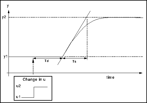
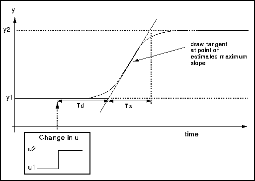
The method is outlined below.

Look at the open loop response of the process to a step change in the manipulated variable.
Evaluate
- The steady-state gain, (y2 - y1) / (u2 - u1)
- The time delay, Td
- The time constant, Ts
The diagram above shows how to obtain these values.
Finally substitute these values into the table below to obtain the relevent controller parameters.

Controller Type Gain Reset Derivative

P Ts / Td - -

PI 0.9 Ts / Td 3.3 Td -

PID 1.2 Ts / Td 2.0 Td 0.5 Td

Controller Type	Gain	Reset	Derivative
P	Ts / Td	-	-
PI	0.9 Ts / Td	3.3 Td	-
PID	1.2 Ts / Td	2.0 Td	0.5 Td

The Gain evaluated above is the product of the controller gain setting,

and the process steady state gain, G.

Gain =

* G

Therefore by substituting all the values in for the above and re-arranging we get the following values for the controller parameters:

Controller Type	Controller Gain,	Reset	Derivative
P	(Ts ) / (Td )	-	-
PI	(0.9 Ts ) / (Td )	3.3 Td	-
PID	(1.2 Ts ) / (Td )	2.0 Td	0.5 Td

Advantages of this method are

Only a single experimental test is needed.
It does not require trial and error
The controller settings are easily calculated.

However there are also Disadvantages

Experiment is under open loop response and so disturbances may affect the results.
Results tend to be oscillatory.
Does not work well for complex responses - leads to inaccurate tuning model.

Controlling Real Processes

In the real world, unfortunately, the response of a process to a change in one of its inputs seldom follows the first-order case required for the Z-N tuning.

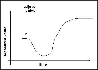
If we are lucky it may be similar in form but different in detail as shown below.

In this case the tangent should be drawn at the point where the slope of the response is steepest. Now we have estimates for the parameters and it may be necessary to change them in order to get the optimum values. To do this it is possible to use a model of the process and controller to see the effect of altering the control parameters. There is the chance to do this in the case study section.

However if we are unlucky the response may be like this...

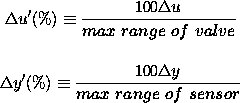
... in which case it is very difficult to control and it may not be possible using a PI controller.

Gains for Real Processes and Controllers

In a process the measurement y is strictly speaking a dimensioned quantity: temperature, pressure, flow etc.

The adjustment u is usually a flow, so that the process gain, , will in general have odd dimensions! This also makes it hard to interpret or compare gain values.

In practice, both measurement and adjustment have a maximum range determined by the measuring instrument or valve. It is best to work with scaled quantities always expressed as a fraction or percentage of range, e.g.

As indicated these values are percentages and so are dimensionless values between 0 and 100. Thus it is possible to define a dimensionless gain for the process as

If the value of the gain is large, say 100, then this means that the change in y is 100 times greater than the corresponding change in u. This could lead to y going out of bounds or else the change in u being very restrictive.

Alternatively, if the gain is very small, say 0.01, then for a large change in u there is hardly any response in y.

What is required is a gain of around 1. This enables both input and output to be used to their full ranges which in turn improves the controllability.

So if this definition of the gain is used it is clear from a glance if a suitable value has been obtained or not. In this case simply use the value of the gain from the first table above along with the dimensionless process gain above to obtain the dimensionless controller gain.

In practice a controller does not want to deal with meaningless dimensions when asking for the value of the gain. Therefore a parameter known as the Proportional Band is used instead.

Firstly remember that you have a value of the dimensionless gain for the controller as evaluated above.

Now we define the Proportional Band, P, as the reciprocal of the dimensionless controller gain.

Remember that when specifying a controller setting, always use dimensionless gain or proportional band.

Return to Start of Module 2.4: Controller Design and System Modelling