There are two ways of approaching the problem of obtaining a mathematical representation or model of a chemical process, or indeed anything.
We will describe briefly some rules for constructing this type of model which help to ensure that if the modeller's understanding of the problem is correct then a correct model will be obtained.
This is a so-called `black box' or `input-output' model, which seeks only to reproduce the behaviour of the system's output in response to changes in its setpoint or inputs. The mathematical form chosen may bear no relation to the form of the equations which truly describe the system. As a result, such models must be used with the greatest care under conditions in the least bit different from those at which the original parameters were determined.
The advantage of such 'arbitrary' models is that they can be developed with little or no knowledge of the system to be represented, and hence complicated systems can be modelled quickly.
Input-output models form the basis of most classical process control theory. They are usually subdivided according to whether they have one or more than one input and/or output. We will consider initially only single input, single output (SISO) models, although some ideas associated with multiple input-output models will be touched on elsewhere in the course.
The basic SISO model can be thought of as relating an output y to an input u. In general both of these quanties will change with time, the model must represent how y responds to changes in its input or inputs.
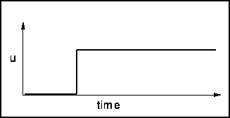
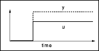
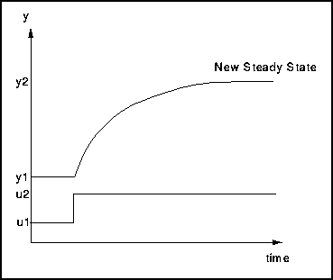
Suppose an input u is given a step change at some time, as shown in the figure.
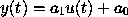
In the above equation
 is called the Gain of the process or
model.
is called the Gain of the process or
model.
is as before the gain, and
 is called the
Time Constant of the equation, system or model.
Because it is described by a single first order o.d.e. this is
called a First Order model, system, lag or response.
The interpretation of these parameters is described below.
is called the
Time Constant of the equation, system or model.
Because it is described by a single first order o.d.e. this is
called a First Order model, system, lag or response.
The interpretation of these parameters is described below.

Models of such systems can be assembled as networks of the elements as shown below.
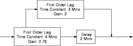
Analytical and numerical techniques are available to work with models constructed in this way.
Classical control theory constructs all its models from sets of
linear ordinary differential equations. (The instantaneous response
is the limiting case of the the o.d.e. where
is zero, and
the plug flow delay, like the plug flow reactor, is the limit of an
infinite number of first order lags.)
There is no good physical reason why a real process should be well represented by such a set of equations, except that in the limit of infinitesimally small changes, all nonlinear equations approximate to linear ones.
However, the theoretical advantage of linear representation is twofold. Firstly, the whole system may be represented by o.d.e.s, whereas if there were any nonlinear algebraic equations a mixed set of differential-algebraic equations would be required. Further, a system of linear differential equations always has an analytical solution, but more particularly, is amenable to various other types of analysis which cannot be performed on nonlinear equations. The tuning methods for controllers described later make use of this type of analysis to obtain generalised equations for suitable controller settings in terms of parameters of a process model written in terms of the above three types of behaviour. This is not possible for nonlinear systems.
It should be stressed that if we wish to simulate the behaviour of a process, which requires only the solution of the relevant equations, and not their analysis, then there is no particular point in approximating it with this type of simplified approximate model. A `real' model should be constructed, as discussed later, and solved.
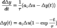
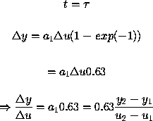
Let us look again at the differential equation which describes first order behaviour.
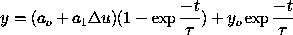
 is the size of the step change in
u at t= 0
is the size of the step change in
u at t= 0
Note that a graph of this equation gives the response curve shown above under the section on the lag response.
The first thing to consider is What is the Change in y
is known as the gain. It tells us how much
the output variable will change per unit change in the input variable.
A large gain implies a large change in y for a given change in
u and
hence leads to a quicker response.
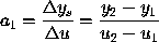
To calculate its value we have to consider the system going from one steady state value to another. Thus we can see what effect a change in u has on the value of y.
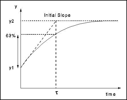
After the system has settled down following the step disturbance


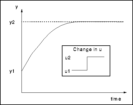
is the time constant for the process. This
is related to the speed of response of the system. The diagram below
shows a graphical method of evaluating its value.
Note that this is also the time taken for the output value to travel 63% of the distance to its new value.
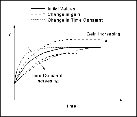
Finally, how does the response change when
and
are altered but the
change in u stays the same?
The diagram below shows that changing
alters the slope of the
initial slope and changing
alters the final steady state.